Visual Examples of Threedx Forecasts

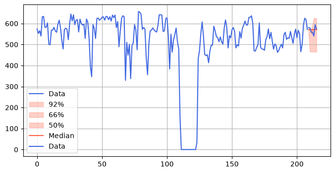
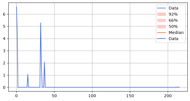
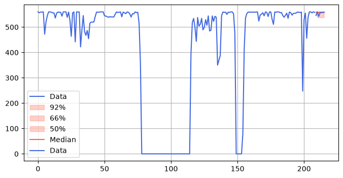
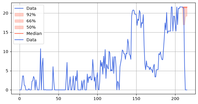
Visualizations of forecasts along with their input time series are often the most interesting part about a paper reporting on new methods. So let’s take a look at some Threedx forecasts for some of the datasets included in the corpus on which the Chronos models were trained, available on Hugging Face. That makes it easy to load the data by not doing much more than importing datasets.

import datasets
import numpy as np
import threedx as tdx
from threedx.graphics import plot_forecast

# Without tuning the parameters to a given use case, we can define the
# parameter grid once upfront and re-use it across datasets and time series.
parameter_grid = tdx.initialize_parameters_at_random(
    size=5000,
    seed=72,
    include_edge_cases=True,
)

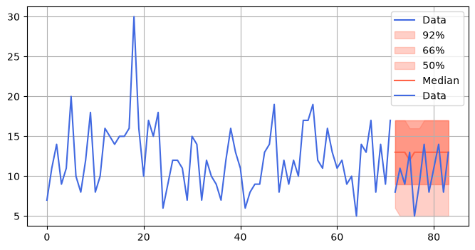
Car Parts

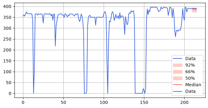
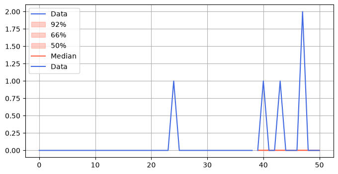
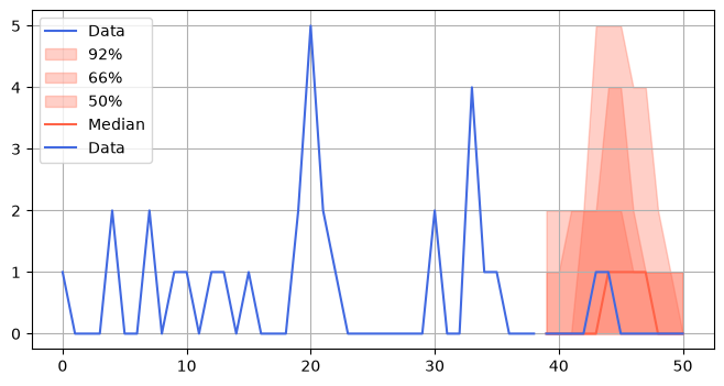
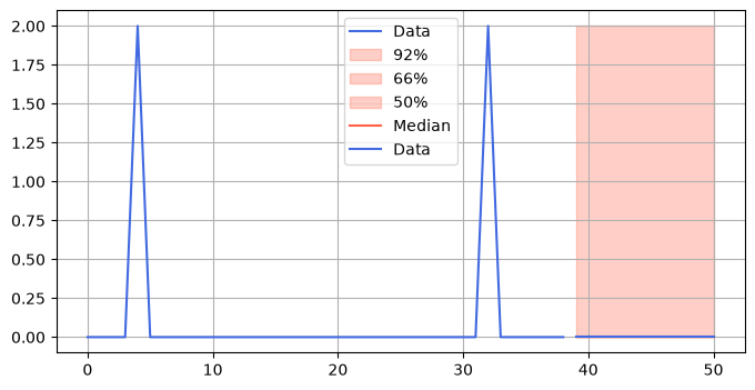
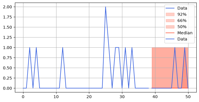
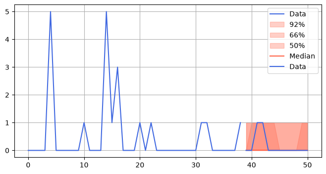
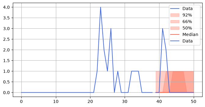
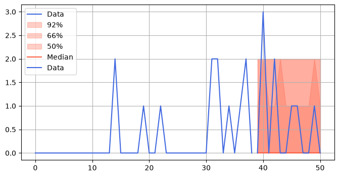
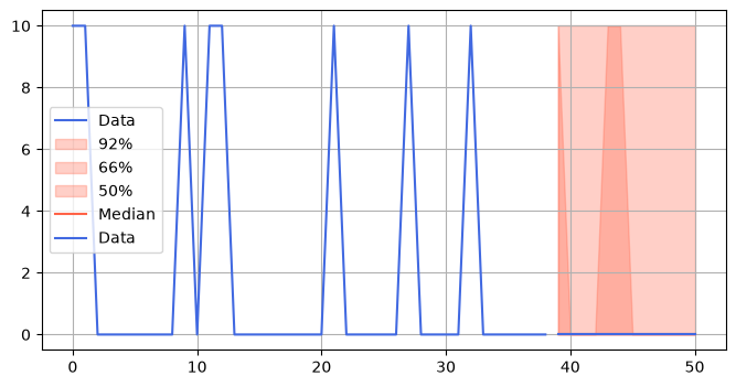
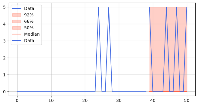
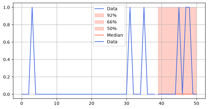
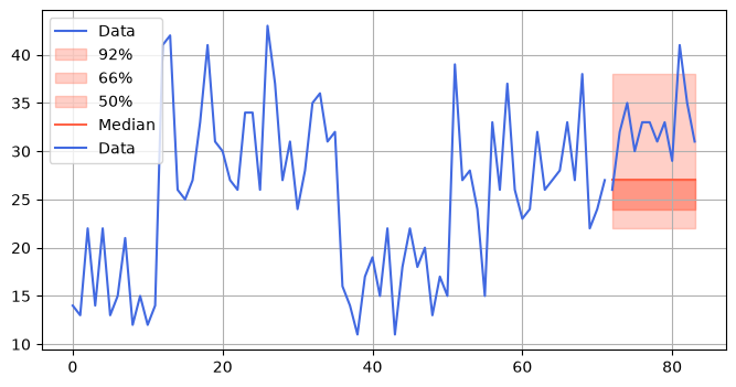
The Car Parts dataset is a classic example of intermittent time series. Very intermittent time series. The observations are recorded on a monthly basis for a couple of years. There are 2674 series.

Assume period_length=12 and forecast the last observed period (twelve months).

ds_car_parts = datasets.load_dataset("autogluon/chronos_datasets", "monash_car_parts", split="train")
ds_car_parts.set_format("numpy")

print(f"{len(ds_car_parts)=}")

Warning: You are sending unauthenticated requests to the HF Hub. Please set a HF_TOKEN to enable higher rate limits and faster downloads.

len(ds_car_parts)=2674

rng = np.random.default_rng(seed=97)
example_series_indices = rng.choice(len(ds_car_parts), size=10)

for i in example_series_indices:
    y_train = ds_car_parts[i]["target"][:-12]
    y_test = ds_car_parts[i]["target"][-12:]

    model = tdx.Threedx(
        period_length=12,
        parameter_grid=parameter_grid,
    )

    model = model.fit(y=y_train, loss=tdx.rmse)

    sample_paths = model.predict(
        horizon=y_test.size,
        n_samples=2501,
        observation_driven=True,
        draw=None,
        seed=823
    )

    plot_forecast(
        forecast=sample_paths,
        y=y_train,
        y_future=y_test
    )

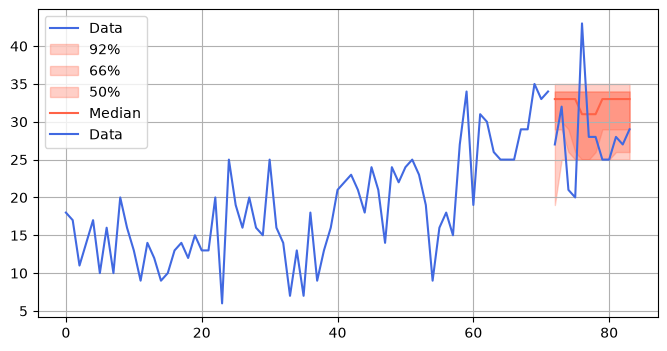
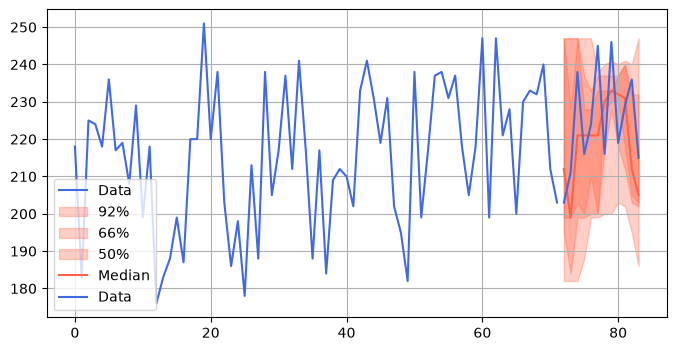
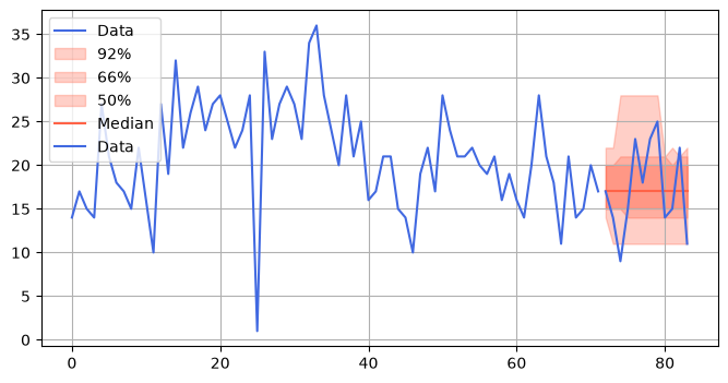
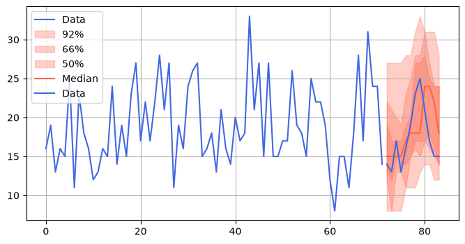
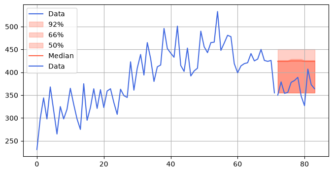
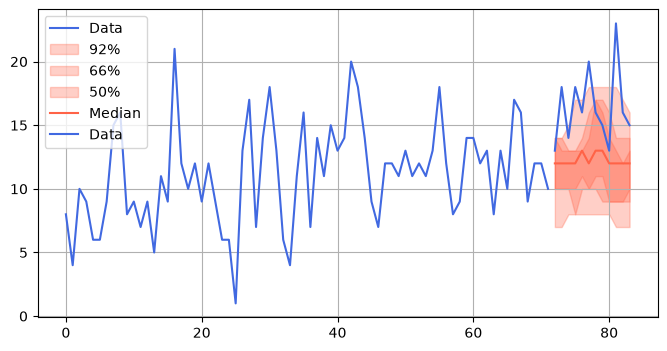
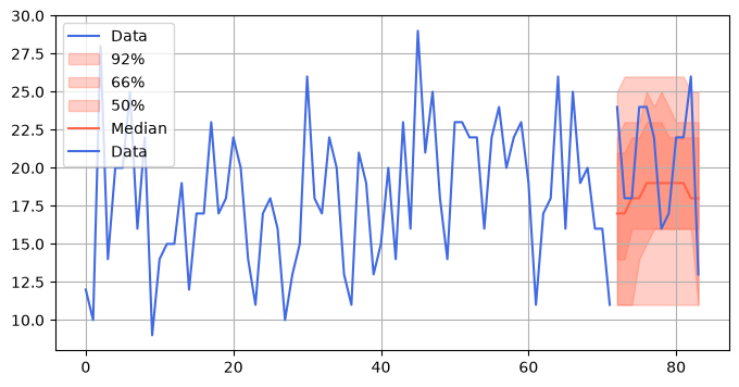
Hospital

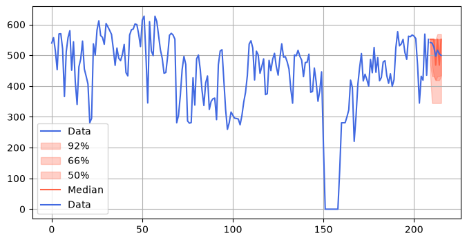
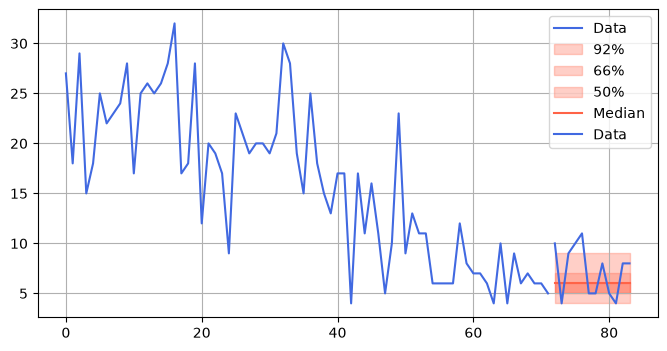
The 767 time series were originally sourced by Hyndman et al. for the “Forecasting with Exponential Smoothing: The State Space Approach” book. From the data’s description in the expsmooth R package:

Monthly patient count for products that are related to medical problems. There are 767 time series that had a mean count of at least 10 and no zeros.

Just like for the Car Parts above, assume period_length=12 and forecast the last observed period (twelve months).

ds_hospital = datasets.load_dataset("autogluon/chronos_datasets", "monash_hospital", split="train")
ds_hospital.set_format("numpy")

print(f"{len(ds_hospital)=}")

len(ds_hospital)=767

rng = np.random.default_rng(seed=442)
example_series_indices = rng.choice(len(ds_hospital), size=10)

for i in example_series_indices:
    y_train = ds_hospital[i]["target"][:-12]
    y_test = ds_hospital[i]["target"][-12:]

    model = tdx.Threedx(
        period_length=12,
        parameter_grid=parameter_grid,
    )

    model = model.fit(y=y_train, loss=tdx.rmse)

    sample_paths = model.predict(
        horizon=y_test.size,
        n_samples=2501,
        observation_driven=True,
        draw=None,
        seed=823
    )

    plot_forecast(
        forecast=sample_paths,
        y=y_train,
        y_future=y_test
    )

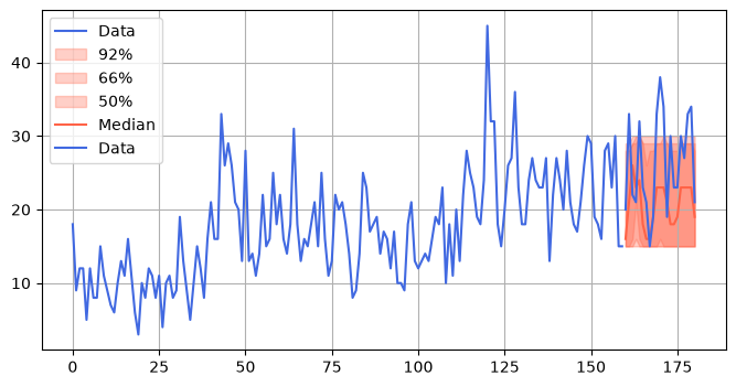
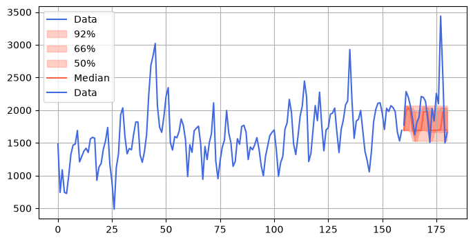
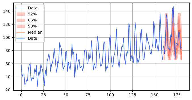
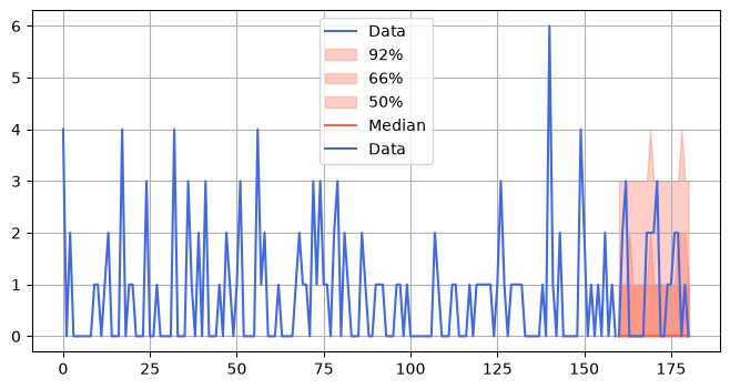
Uber TLC Daily

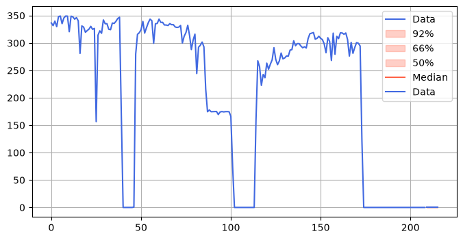
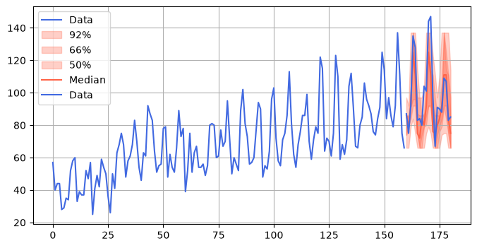
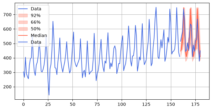
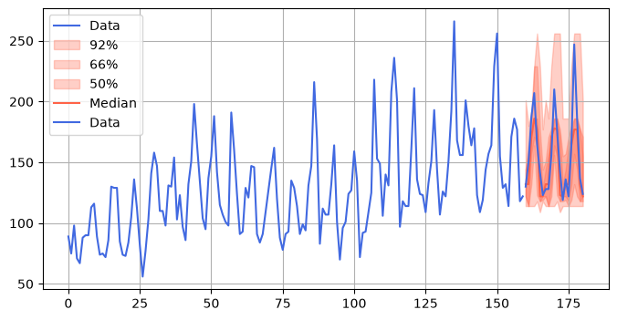
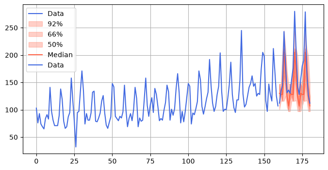
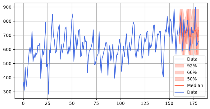
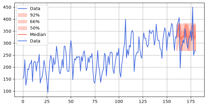
Some daily time series related to data published by New York’s Taxi and Limousine Commission (TLC) about Uber, sourced originally by FiveThirtyEight.

Assume a weekly seasonal component with period_length=7 and predict three periods (21 days) into the future.

ds_uber_daily = datasets.load_dataset("autogluon/chronos_datasets", "uber_tlc_daily", split="train")
ds_uber_daily.set_format("numpy")

print(f"{len(ds_uber_daily)=}")

len(ds_uber_daily)=262

rng = np.random.default_rng(seed=44)
example_series_indices = rng.choice(len(ds_uber_daily), size=10)

for i in example_series_indices:
    y_train = ds_uber_daily[i]["target"][:-21]
    y_test = ds_uber_daily[i]["target"][-21:]

    model = tdx.Threedx(
        period_length=7,
        parameter_grid=parameter_grid,
    )

    model = model.fit(y=y_train, loss=tdx.rmse)

    sample_paths = model.predict(
        horizon=y_test.size,
        n_samples=2501,
        observation_driven=True,
        draw=None,
        seed=823
    )

    plot_forecast(
        forecast=sample_paths,
        y=y_train,
        y_future=y_test
    )

Wind Farms Daily

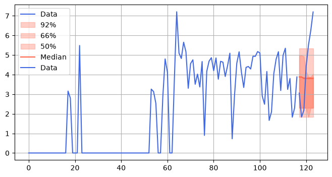
Daily observations on 337 wind power production time series aggregated from a dataset included in the Monash Time Series Forecasting Repository. The time series are fairly long and include missing values in within the first 150 days (observations).

Assume period_length=7 and predict the last period (seven days). Impute missing values with zero if there are any (as done in the second published version of the dataset).

ds_wind_farms_daily = datasets.load_dataset("autogluon/chronos_datasets", "wind_farms_daily", split="train")
ds_wind_farms_daily.set_format("numpy")

print(f"{len(ds_wind_farms_daily)=}")

len(ds_wind_farms_daily)=337

rng = np.random.default_rng(seed=928)
example_series_indices = rng.choice(len(ds_wind_farms_daily), size=10)

for i in example_series_indices:
    y_train = ds_wind_farms_daily[i]["target"][150:-7]
    y_test = ds_wind_farms_daily[i]["target"][-7:]

    model = tdx.Threedx(
        period_length=7,
        parameter_grid=parameter_grid,
    )

    model = model.fit(
        y=np.nan_to_num(y_train, nan=0.0),
        loss=tdx.rmse
    )

    sample_paths = model.predict(
        horizon=y_test.size,
        n_samples=2501,
        observation_driven=True,
        draw=None,
        seed=488
    )

    plot_forecast(
        forecast=sample_paths,
        y=y_train,
        y_future=y_test
    )