Get Started

To do anything, you require a time series to predict. Import numpy to generate a fairly short time series of monthly, non-negative observations with a strong yearly seasonality.

import numpy as np

n_obs = 65
period_length = 12
rng = np.random.default_rng(seed=512)

_y = rng.poisson(
    lam=np.maximum(
        0.1,
        1 + 10 * np.sin(2 * np.pi * np.arange(6, 6 + n_obs) / period_length)
    ),
    size=n_obs
)

y = _y[:(n_obs-period_length)]
y_future = _y[(n_obs-period_length):]

Assuming you have already installed Threedx, continue by importing it. This loads all components necessary to fit a first model.

import threedx as tdx

Initialize the threedx Model

The standard interface to fit and predict with Threedx is by initializing a Threedx object which provides .fit() and .predict() methods.

During intialization, you have to provide the parameter grid that Threedx will perform grid search optimization over. The threedx.initialize submodule provides several functions that create such a grid, but you can define the grid in any way you like as long as it is a two-dimensional numpy array with three columns and floating values ranging from 0 to 1.

For example, we can create a grid at random using threedx.initialize.initialize_parameters_at_random():

grid = tdx.initialize_parameters_at_random(
    size=2500,
    seed=729,
    include_edge_cases=True
)

The resulting grid looks as follows. Note that by default include_edge_cases=True, meaning that despite drawing the grid randomly, the first couple of rows are deterministically set to special cases at the boundary of the allowed value range.

# The parameter grid over which the parameters will be optimized:
np.round(grid, 3)

array([[1.   , 0.   , 0.   ],
       [0.   , 0.   , 0.   ],
       [0.   , 1.   , 0.   ],
       ...,
       [0.29 , 0.358, 0.877],
       [0.284, 0.442, 0.881],
       [0.318, 0.787, 0.241]], shape=(2500, 3))

With the parameter grid at hand, go ahead and initialize the Threedx object. Besides the parameter grid, specify the period length of the time series’ dominant seasonal component. In this case, set period_length=12 as the monthly data could exhibit a yearly seasonality.

model = tdx.Threedx(period_length=12, parameter_grid=grid)

Fit the threedx Model to Data

Call the .fit() method to train the initialized model on your time series. Threedx requires you to specify the loss function that will be optimized during training.

Below we use one of those provided in threedx.loss, but you can specify your own. They only need to match the threedx.loss.Loss protocol: Take a one-dimensional array of observations, a one-dimensional array of predictions, and return a scalar as loss.

model = model.fit(
    y=y,
    loss=tdx.mae # Specify your preferred loss function
)

Predict Using the Fitted Model

Threedx forecasts come in the form of sample paths. Compared to marginal quantiles, sample paths offer more flexibility for downstream optimization that might rely on arbitrary sums over forecast horizon spans. And if quantiles or point forecasts do suffice, the sample paths can of course be aggregated to them.

Use the .predict() method to draw sample paths.

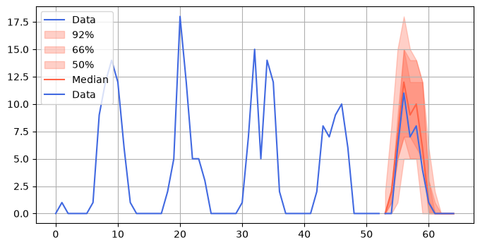
By default, sample paths are generated by sampling from weighted past observations (observation_driven=True):

sample_paths_from_observations = model.predict(
    horizon=period_length,
    n_samples=2501,
    observation_driven=True,
    draw=None,
    seed=388
)

Being able to draw sample paths based on observations is a unique feature of Threedx. The more common method of drawing sample paths via innovations learned from residuals is an alternative option (observation_driven=False). To use it, specify how innovations should be generated by passing a Callable to draw.

Below, innovations are generated via threedx.innovations.draw_bootstrap() as bootstrap samples from fitted residuals. See threedx.innovations for alternatives or specify your own function following the threedx.innovations.Draw protocol.

sample_paths_from_innovations = model.predict(
    horizon=period_length,
    n_samples=2501,
    observation_driven=False,
    draw=tdx.draw_bootstrap,
    seed=512
)

Threedx comes with helper functions to plot forecasts as marginal quantiles along with past (and optionally future) observations. This requires the optional graphics dependencies (i.e. matplotlib) to be installed via threedx[graphics].

from threedx.graphics import plot_forecast

plot_forecast(
    forecast=sample_paths_from_observations,
    y=y,
    y_future=y_future
)

plot_forecast(
    forecast=sample_paths_from_innovations,
    y=y,
    y_future=y_future
)

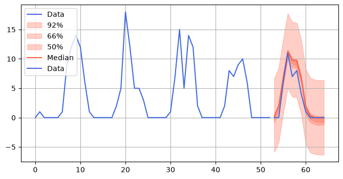
While the median predictions from both observation-driven and innovation-driven forecasts are similar, the forecast intervals differ heavily: The innovation-driven predictions are not constrained to non-negative values and cannot account for the heteroskedastic errors.

Parameters of the Fitted Model

At the beginning of the notebook, you started by defining a parameter grid over which the model will be optimized. The model was fitted on the following optimal parameters given your chosen loss function and past observations:

print(f"{model.best_alpha=}")
print(f"{model.best_alpha_seasonal=}")
print(f"{model.best_alpha_seasonal_decay=}")

model.best_alpha=np.float64(0.0020794643341743354)
model.best_alpha_seasonal=np.float64(0.8592539151871426)
model.best_alpha_seasonal_decay=np.float64(0.1156035225969444)

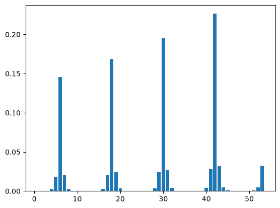
Threedx predicts by projecting these three parameters into a weight-space in which a weight is assigned to every past observation. This allows Threedx to draw sample paths by sampling past observations according to the weight assigned to them. A mean prediction is nothing but the linear combination of weights and past observations.

The weights assigned to the time series on which the model is fitted can be inspected using the .weights() method:

np.round(model.weights(), 4)

array([0.000e+00, 0.000e+00, 4.000e-04, 2.500e-03, 1.800e-02, 1.452e-01,
       2.050e-02, 2.900e-03, 4.000e-04, 1.000e-04, 0.000e+00, 0.000e+00,
       0.000e+00, 1.000e-04, 4.000e-04, 2.900e-03, 2.090e-02, 1.684e-01,
       2.370e-02, 3.300e-03, 5.000e-04, 1.000e-04, 0.000e+00, 0.000e+00,
       0.000e+00, 1.000e-04, 5.000e-04, 3.400e-03, 2.420e-02, 1.952e-01,
       2.750e-02, 3.900e-03, 5.000e-04, 1.000e-04, 0.000e+00, 0.000e+00,
       0.000e+00, 1.000e-04, 6.000e-04, 3.900e-03, 2.810e-02, 2.263e-01,
       3.190e-02, 4.500e-03, 6.000e-04, 1.000e-04, 0.000e+00, 0.000e+00,
       0.000e+00, 1.000e-04, 6.000e-04, 4.600e-03, 3.260e-02])

Use weights_threedx() to produce a weight vector given a set of parameters independent from a model:

np.round(
    tdx.weights_threedx(
        alpha=model.best_alpha,
        alpha_seasonal=model.best_alpha_seasonal,
        alpha_seasonal_decay=model.best_alpha_seasonal_decay,
        n=y.size,
        period_length=period_length
    ), 4
)

array([0.000e+00, 0.000e+00, 4.000e-04, 2.500e-03, 1.800e-02, 1.452e-01,
       2.050e-02, 2.900e-03, 4.000e-04, 1.000e-04, 0.000e+00, 0.000e+00,
       0.000e+00, 1.000e-04, 4.000e-04, 2.900e-03, 2.090e-02, 1.684e-01,
       2.370e-02, 3.300e-03, 5.000e-04, 1.000e-04, 0.000e+00, 0.000e+00,
       0.000e+00, 1.000e-04, 5.000e-04, 3.400e-03, 2.420e-02, 1.952e-01,
       2.750e-02, 3.900e-03, 5.000e-04, 1.000e-04, 0.000e+00, 0.000e+00,
       0.000e+00, 1.000e-04, 6.000e-04, 3.900e-03, 2.810e-02, 2.263e-01,
       3.190e-02, 4.500e-03, 6.000e-04, 1.000e-04, 0.000e+00, 0.000e+00,
       0.000e+00, 1.000e-04, 6.000e-04, 4.600e-03, 3.260e-02])

As the decimal values are a bit hard to read, this is what they look like as a column chart:

import matplotlib.pyplot as plt

plt.bar(
    x=np.arange(1, y.size+1),
    height=model.weights()
)

<BarContainer object of 53 artists>