From Parameters to Weights

A Threedx model is defined by its three parameters: alpha, alpha_seasonal, and alpha_seasonal_decay. Together, the three parameters define the weights that a Threedx model assigns to past observations when calculating a forecast. To understand the meaning of the parameters and their impact on a Threedx forecast, you need to understand how the three parameters are projected into weights space.

import matplotlib.pyplot as plt
import numpy as np
import threedx as tdx

Understanding the Individual Parameters

The best way to understand how the three parameters interact is to first understand how they work individually. Each of the parameters can be used to derive weights; a Threedx model in the end only combines the three individual weight vectors into a combined one.

Common Characteristics

Before looking at each parameter individually, keep in mind that the following characteristics hold for each of the three parameters:

• Each parameter can take values in the range of [0, 1]

• Threedx weight vectors always sum up to 1

Understanding alpha

The alpha parameter creates exponential weights just like the alpha parameter in Simple Exponential Smoothing, following the update equation:

w_t = alpha * ((1-alpha) ** (t-1))

You can generate a vector of n exponential smoothing weights using alpha as follows:

tdx.weights_exponential(alpha=0.1, n=5)

array([0.16021587, 0.17801763, 0.19779737, 0.21977485, 0.24419428])

To align with time series, Threedx weight vectors always range from the weight for the oldest observation on the left, to the weight for the most recent observation on the right. Exponential weights specifically assign the largest weight to the most recent observation and decrease monotonically from there to the smallest weight being assigned to the oldest observation.

Note that Threedx weight vectors are always standardized to sum to one. This has a small impact if alpha or n are large. In the example above, however, the most recent weight is 0.24 instead of 0.1 because the smoothing factor alpha is small (implying little smoothing) while n, too, is small.

Non-normalized weights would look as follows (note that the most recent weight is equal to alpha):

n = 5
alpha = 0.1

weights_non_normalized = alpha * ((1 - alpha) ** np.arange(n)[::-1])

print(f"{weights_non_normalized=}")
print(f"{weights_non_normalized.sum()=}")

weights_non_normalized=array([0.06561, 0.0729 , 0.081  , 0.09   , 0.1    ])
weights_non_normalized.sum()=np.float64(0.40951000000000004)

With sufficiently large n, normalization is barely needed as the sum of exponential weights approaches one:

n = 100
weights_non_normalized_large_n = alpha * ((1 - alpha) ** np.arange(n)[::-1])

print(f"{weights_non_normalized_large_n.sum()=}")

weights_non_normalized_large_n.sum()=np.float64(0.9999734386011125)

At the one extreme of alpha=0, weights are distributed uniformly and would result in a forecast equal to the simple average of past observations:

tdx.weights_exponential(alpha=0., n=5)

array([0.2, 0.2, 0.2, 0.2, 0.2])

At the other extreme of alpha=1, all weight is assigned to the most recent observation and would thus result in a naive forecast:

tdx.weights_exponential(alpha=1., n=5)

array([0., 0., 0., 0., 1.])

All other alpha values interpolate smoothly between the two extremes:

print(f"alpha=0.00: {tdx.weights_exponential(alpha=0.00, n=5)}")
print(f"alpha=0.01: {tdx.weights_exponential(alpha=0.01, n=5)}")
print(f"alpha=0.10: {tdx.weights_exponential(alpha=0.10, n=5)}")
print(f"alpha=0.50: {tdx.weights_exponential(alpha=0.50, n=5)}")
print(f"alpha=0.90: {tdx.weights_exponential(alpha=0.90, n=5)}")
print(f"alpha=0.99: {tdx.weights_exponential(alpha=0.99, n=5)}")
print(f"alpha=1.00: {tdx.weights_exponential(alpha=1.00, n=5)}")

alpha=0.00: [0.2 0.2 0.2 0.2 0.2]
alpha=0.01: [0.1960002 0.19798   0.1999798 0.2019998 0.2040402]
alpha=0.10: [0.16021587 0.17801763 0.19779737 0.21977485 0.24419428]
alpha=0.50: [0.03225806 0.06451613 0.12903226 0.25806452 0.51612903]
alpha=0.90: [9.00009e-05 9.00009e-04 9.00009e-03 9.00009e-02 9.00009e-01]
alpha=0.99: [9.9e-09 9.9e-07 9.9e-05 9.9e-03 9.9e-01]
alpha=1.00: [0. 0. 0. 0. 1.]

Understanding alpha_seasonal_decay

While normally the third parameter, it makes sense to continue with alpha_seasonal_decay for the purpose of this tutorial. Both alpha_seasonal and alpha_seasonal_decay extend the idea of exponential smoothing weights to seasonal time series. To generate weight vectors with either of the two parameters, it’s necessary to supply an additional period_length argument to define the expected period length of the time series’ seasonal component.

Consequently, a weight vector based on alpha_seasonal_decay can be generated as follows (here for a weekly period length as could be used for daily observations):

tdx.weights_seasonal_decay(alpha=0.1, n=35, period_length=7)

array([0.02288798, 0.02288798, 0.02288798, 0.02288798, 0.02288798,
       0.02288798, 0.02288798, 0.02543109, 0.02543109, 0.02543109,
       0.02543109, 0.02543109, 0.02543109, 0.02543109, 0.02825677,
       0.02825677, 0.02825677, 0.02825677, 0.02825677, 0.02825677,
       0.02825677, 0.03139641, 0.03139641, 0.03139641, 0.03139641,
       0.03139641, 0.03139641, 0.03139641, 0.0348849 , 0.0348849 ,
       0.0348849 , 0.0348849 , 0.0348849 , 0.0348849 , 0.0348849 ])

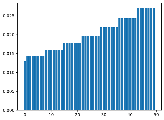
The seasonal decay weights steered by alpha_seasonal_decay only change outside of seasonal periods or across seasonal periods, but are constant within seasonal periods. Starting from the most recent observation (the last weight in the vector), weights are constant for period_length weights, then change to a new value for the next period_length weights, and so on.

Across periods, weights decrease again exponentially. This fact is a bit hidden in the above example due to the standardization of the weight vector to sum to one. It can be recovered by considering the unique values and re-normalizing them. They then match the exponential weights where alpha=alpha_seasonal_decay.

weights_seasonal_decay_unique = np.unique(
    tdx.weights_seasonal_decay(alpha=0.1, n=35, period_length=7)
)

weights_seasonal_decay_unique_normalized = \
    weights_seasonal_decay_unique / weights_seasonal_decay_unique.sum()

print(f"{weights_seasonal_decay_unique=}")
print(f"{weights_seasonal_decay_unique_normalized=}")
print(f"{tdx.weights_exponential(alpha=0.1, n=5)=}")

weights_seasonal_decay_unique=array([0.02288798, 0.02543109, 0.02825677, 0.03139641, 0.0348849 ])
weights_seasonal_decay_unique_normalized=array([0.16021587, 0.17801763, 0.19779737, 0.21977485, 0.24419428])
tdx.weights_exponential(alpha=0.1, n=5)=array([0.16021587, 0.17801763, 0.19779737, 0.21977485, 0.24419428])

Or set period_length=1 to arrive at the same conclusion:

print(f"{tdx.weights_seasonal_decay(alpha=0.1, n=5, period_length=1)=}")

tdx.weights_seasonal_decay(alpha=0.1, n=5, period_length=1)=array([0.16021587, 0.17801763, 0.19779737, 0.21977485, 0.24419428])

The fact that weights only change across periods results in a step function pattern that becomes even more obvious when plotting the weight vectors:

plt.bar(
    x=np.arange(50),
    height=tdx.weights_seasonal_decay(alpha=0.1, n=50, period_length=7),
)

<BarContainer object of 50 artists>

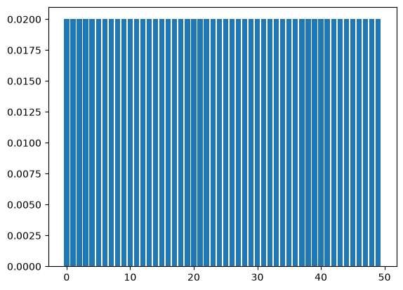
At the extreme of alpha_seasonal_decay=0., weights are perfectly uniform:

plt.bar(
    x=np.arange(50),
    height=tdx.weights_seasonal_decay(alpha=0.0, n=50, period_length=7),
)

<BarContainer object of 50 artists>

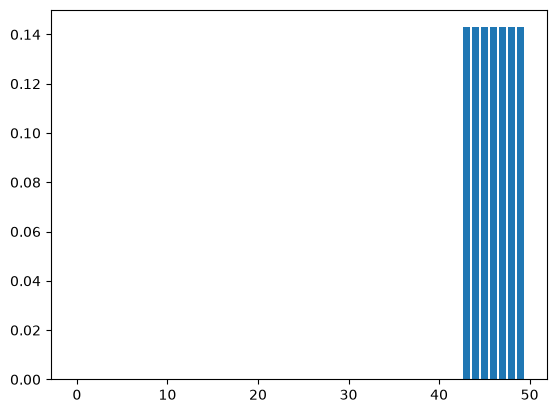
At the other extreme of alpha_seasonal_decay=1.0, all weight is assigned to the most recent period (and within that period uniformly). The resulting weight vector would generate a latest-period-average forecast.

plt.bar(
    x=np.arange(50),
    height=tdx.weights_seasonal_decay(alpha=1.0, n=50, period_length=7),
)

<BarContainer object of 50 artists>

Understanding alpha_seasonal

Like alpha_seasonal_decay, alpha_seasonal transforms into weights that account for a seasonal component in time series. While alpha_seasonal_decay transforms into weights that vary across periods, alpha_seasonal transforms into weights that vary within a seasonal period but stay constant across periods.

This is understood easiest by looking at the resulting weight vector:

plt.bar(
    x=np.arange(50),
    height=tdx.weights_seasonal(alpha=0.1, n=50, period_length=7),
)

<BarContainer object of 50 artists>

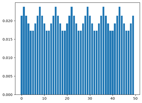
Within a given period, alpha_seasonal distributes weights by assigning the most weight to the observation at the beginning of the period and the least weight to observations in the middle of a period. At the extreme of alpha_seasonal=1, this results in a seasonal average forecast. At values between zero and one, this results in forecasts primarily based on past observations that are similar to the predicted point in time in terms of their position within the seasonal period.

print(f"alpha=0.00: {tdx.weights_seasonal(alpha=0.00, n=5, period_length=5)}")
print(f"alpha=0.01: {tdx.weights_seasonal(alpha=0.01, n=5, period_length=5)}")
print(f"alpha=0.10: {tdx.weights_seasonal(alpha=0.10, n=5, period_length=5)}")
print(f"alpha=0.50: {tdx.weights_seasonal(alpha=0.50, n=5, period_length=5)}")
print(f"alpha=0.90: {tdx.weights_seasonal(alpha=0.90, n=5, period_length=5)}")
print(f"alpha=0.99: {tdx.weights_seasonal(alpha=0.99, n=5, period_length=5)}")
print(f"alpha=1.00: {tdx.weights_seasonal(alpha=1.00, n=5, period_length=5)}")

alpha=0.00: [0.2 0.2 0.2 0.2 0.2]
alpha=0.01: [0.20242095 0.20039675 0.19839278 0.19839278 0.20039675]
alpha=0.10: [0.22624434 0.20361991 0.18325792 0.18325792 0.20361991]
alpha=0.50: [0.4 0.2 0.1 0.1 0.2]
alpha=0.90: [0.81967213 0.08196721 0.00819672 0.00819672 0.08196721]
alpha=0.99: [9.80199961e-01 9.80199961e-03 9.80199961e-05 9.80199961e-05
 9.80199961e-03]
alpha=1.00: [1. 0. 0. 0. 0.]

Understanding the Combined Parameters

The final weight vector used by a Threedx model is a combination of the three individual parameters’ weight vectors. Consequently, it will exhibit a combination of the three individual weight vectors’ characteristics. This is again most transparent when plotting the weights:

weights_threedx = tdx.weights_threedx(
    alpha=0.01,
    alpha_seasonal=0.1,
    alpha_seasonal_decay=0.1,
    n=50,
    period_length=7
)

plt.bar(x=np.arange(50), height=weights_threedx)

<BarContainer object of 50 artists>

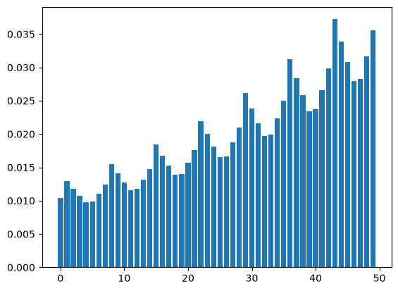
The combined weight vector is simply the product of the three vectors, normalized to sum up to one. The weights generated by tdx.weights_threedx() can be recreated using the three individual weight functions as follows:

combined_weights = \
    tdx.weights_exponential(alpha=0.01, n=50) * \
    tdx.weights_seasonal(alpha=0.1, n=50, period_length=7) * \
    tdx.weights_seasonal_decay(alpha=0.1, n=50, period_length=7)

combined_weights = combined_weights / combined_weights.sum()

print(f"{combined_weights=}")
print(f"{weights_threedx=}")

combined_weights=array([0.01040076, 0.01297015, 0.01179104, 0.01071913, 0.00974466,
       0.00984309, 0.01104724, 0.0123987 , 0.01546165, 0.01405605,
       0.01277823, 0.01161657, 0.01173391, 0.01316937, 0.01478044,
       0.01843177, 0.01675616, 0.01523287, 0.01384806, 0.01398794,
       0.01569915, 0.0176197 , 0.02197244, 0.01997494, 0.01815904,
       0.01650822, 0.01667497, 0.01871489, 0.02100437, 0.02619325,
       0.02381204, 0.02164731, 0.01967937, 0.01987816, 0.02230994,
       0.02503921, 0.03122486, 0.02838623, 0.02580567, 0.0234597 ,
       0.02369666, 0.02659558, 0.02984914, 0.03722302, 0.03383911,
       0.03076283, 0.02796621, 0.02824869, 0.03170448, 0.03558303])
weights_threedx=array([0.01040076, 0.01297015, 0.01179104, 0.01071913, 0.00974466,
       0.00984309, 0.01104724, 0.0123987 , 0.01546165, 0.01405605,
       0.01277823, 0.01161657, 0.01173391, 0.01316937, 0.01478044,
       0.01843177, 0.01675616, 0.01523287, 0.01384806, 0.01398794,
       0.01569915, 0.0176197 , 0.02197244, 0.01997494, 0.01815904,
       0.01650822, 0.01667497, 0.01871489, 0.02100437, 0.02619325,
       0.02381204, 0.02164731, 0.01967937, 0.01987816, 0.02230994,
       0.02503921, 0.03122486, 0.02838623, 0.02580567, 0.0234597 ,
       0.02369666, 0.02659558, 0.02984914, 0.03722302, 0.03383911,
       0.03076283, 0.02796621, 0.02824869, 0.03170448, 0.03558303])

Understanding the Edge Cases

With its three parameters, a Threedx model can fit a wide range of different weights that interpolate between a set of edge cases.

Simple Average Forecast

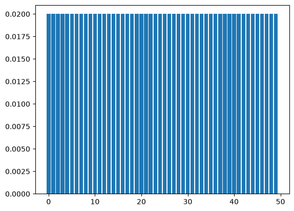
By setting each parameter to zero, a Threedx model assigns weights to past observations that result in a simple average forecast. The weights are perfectly uniform.

weights_simple_average = tdx.weights_threedx(
    alpha=0.,
    alpha_seasonal=0.,
    alpha_seasonal_decay=0.,
    n=50,
    period_length=7
)

plt.bar(x=np.arange(50), height=weights_simple_average)

<BarContainer object of 50 artists>

Naive Forecast

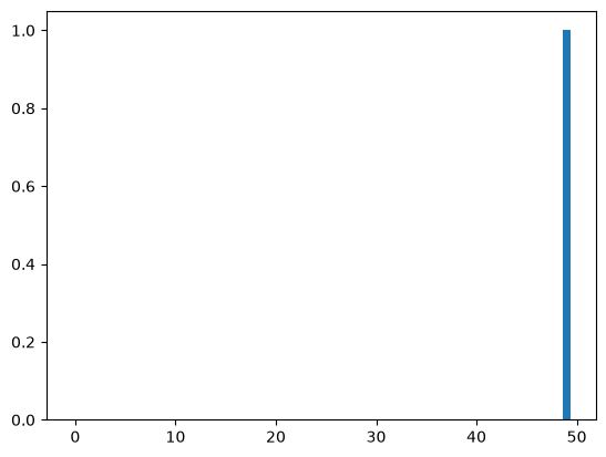
Whenever the alpha parameter is set to one, independent of the other two parameters, all weight will be assigned to the most recent observation. This results in a naive forecast.

weights_naive = tdx.weights_threedx(
    alpha=1.,
    alpha_seasonal=0.,
    alpha_seasonal_decay=0.,
    n=50,
    period_length=7
)

plt.bar(x=np.arange(50), height=weights_naive)

<BarContainer object of 50 artists>

Seasonal Average Forecast

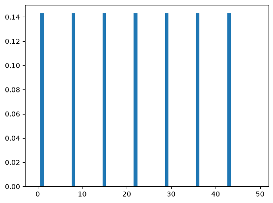
A seasonal average forecast requires uniform weights on the observations k-periods ago, and zero weight on observations in between. This can be achieved by choosing alpha=0 and alpha_seasonal_decay=0 (avoiding decreasing weights) and choosing alpha_seasonal=1 to assign all weight within a period onto a single observation in the period.

weights_seasonal_average = tdx.weights_threedx(
    alpha=0.,
    alpha_seasonal=1.,
    alpha_seasonal_decay=0.,
    n=50,
    period_length=7
)

plt.bar(x=np.arange(50), height=weights_seasonal_average)

<BarContainer object of 50 artists>

Seasonal Naive Forecast

In contrast to the seasonal average, the seasonal naive forecast uses only the most recent period (and within that period the observation a period ago). This means you want extreme decay across periods and thus change to alpha_seasonal_decay=1:

weights_seasonal_naive = tdx.weights_threedx(
    alpha=0.,
    alpha_seasonal=1.,
    alpha_seasonal_decay=1.,
    n=50,
    period_length=7
)

plt.bar(x=np.arange(50), height=weights_seasonal_naive)

<BarContainer object of 50 artists>

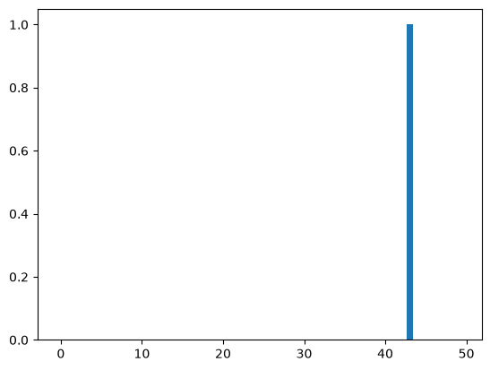
Latest Period Average Forecast

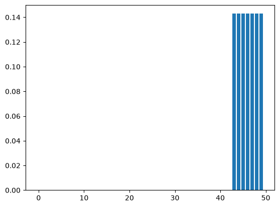
Finally, switch to alpha_seasonal=0 to keep assigning all weight to the most recent period. This will, however, distribute the weight uniformly across all observations within that period. The resulting forecast is the average of the observations in the most recent period.

weights_latest_period_average = tdx.weights_threedx(
    alpha=0.,
    alpha_seasonal=0.,
    alpha_seasonal_decay=1.,
    n=50,
    period_length=7
)

plt.bar(x=np.arange(50), height=weights_latest_period_average)

<BarContainer object of 50 artists>

Choosing the Parameter Grid

You need a solid understanding of how parameters are projected into weight space, and how weights result into forecasts when you define the parameter grid over which a Threedx model is fitted. As shown in the Get Started section, you need to provide a parameter grid when you initialize the Threedx model object.

The threedx.initialize module provides functions that make it easy to define such a grid.

For example, you know understand how to interpret the parameter combinations that the threedx.initialize.initialize_edge_case_parameters() function generates:

tdx.initialize_edge_case_parameters()

array([[1., 0., 0.],
       [0., 0., 0.],
       [0., 1., 0.],
       [0., 1., 1.],
       [0., 0., 1.]])

The edge cases are included per default also when you create a larger set of parameter combinations using initialize_parameters_at_random() or initialize_parameters_in_grid():

tdx.initialize_parameters_at_random(size=10, include_edge_cases=True)

array([[1.        , 0.        , 0.        ],
       [0.        , 0.        , 0.        ],
       [0.        , 1.        , 0.        ],
       [0.        , 1.        , 1.        ],
       [0.        , 0.        , 1.        ],
       [0.44600965, 0.95405379, 0.26779936],
       [0.1737167 , 0.72216041, 0.55418015],
       [0.43663052, 0.7679298 , 0.68672886],
       [0.41652369, 0.5452752 , 0.15716583],
       [0.47342419, 0.89501644, 0.3589646 ]])

But all of these functions are just provided to get you started. You can define the parameter grid in any way you like. Apply the understanding you gained throughout this tutorial to fit a Threedx model over parameters that make sense for your use case.

For example, you could restrict the range of models that Threedx will fit to Simple Exponential Smoothing models by only varying the alpha parameter and setting alpha_seasonal and alpha_seasonal_decay to zero, as follows:

grid_simple_exponential_smoothing = np.zeros((10, 3))
grid_simple_exponential_smoothing[:, 0] = np.arange(0, 1, 0.1)
print(grid_simple_exponential_smoothing)

[[0.  0.  0. ]
 [0.1 0.  0. ]
 [0.2 0.  0. ]
 [0.3 0.  0. ]
 [0.4 0.  0. ]
 [0.5 0.  0. ]
 [0.6 0.  0. ]
 [0.7 0.  0. ]
 [0.8 0.  0. ]
 [0.9 0.  0. ]]