Observation-driven Sample Paths

Threedx generates sample path forecasts observation-driven per default. This is possible because a Threedx model assigns weights to all past observations. Using these weights, the model then samples past observations with replacement to draw sample paths.

Take a closer look by fitting a model using some example data.

Inspect Observation-driven Sample Paths

import numpy as np
import threedx as tdx
from threedx.graphics import plot_forecast
from threedx._data import _load_y

y, _ = _load_y()

model = tdx.Threedx(
    period_length=12,
    parameter_grid=tdx.initialize_parameters_at_random(
        size=2500,
        seed=729,
        include_edge_cases=True
    )
)

model = model.fit(
    y=y,
    loss=tdx.mae
)

The choice of observation_driven=True and draw=None is the default for the .predict() method. Use it to generate sample paths, then visualize them.

sample_paths_from_observations = model.predict(
    horizon=12,
    n_samples=2501,
    observation_driven=True,
    draw=None,
    seed=388
)

plot_forecast(
    forecast=sample_paths_from_observations,
    y=y
)

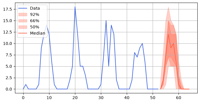
The above plot highlights one immediate advantage of observation-driven forecasts: They are limited to the observed range of values. Here, forecast intervals are limited to non-negative values even though you didn’t supply that constraint to the model. But the largest predicted value is also equal to the largest observed value, 18.

That the sample paths consist only of sampled observations becomes even more obvious when you print the unique observed values and the unique values from sample paths:

print("Unique values in observated time series:")
print(np.unique(y))

print("\nUnique values in sample path forecasts:")
print(np.unique(sample_paths_from_observations))

Unique values in observated time series:
[ 0  1  2  3  5  6  7  8  9 10 12 14 15 18]

Unique values in sample path forecasts:
[ 0.  1.  2.  3.  5.  6.  7.  8.  9. 10. 12. 14. 15. 18.]

As described in Interpret Threedx Forecasts, you can inspect the weights that the fitted model assigns to past observations using the .weights() method. These are the weights applied when sampling past observations with replacement.

np.round(model.weights(), 4)

array([0.000e+00, 0.000e+00, 4.000e-04, 2.500e-03, 1.800e-02, 1.452e-01,
       2.050e-02, 2.900e-03, 4.000e-04, 1.000e-04, 0.000e+00, 0.000e+00,
       0.000e+00, 1.000e-04, 4.000e-04, 2.900e-03, 2.090e-02, 1.684e-01,
       2.370e-02, 3.300e-03, 5.000e-04, 1.000e-04, 0.000e+00, 0.000e+00,
       0.000e+00, 1.000e-04, 5.000e-04, 3.400e-03, 2.420e-02, 1.952e-01,
       2.750e-02, 3.900e-03, 5.000e-04, 1.000e-04, 0.000e+00, 0.000e+00,
       0.000e+00, 1.000e-04, 6.000e-04, 3.900e-03, 2.810e-02, 2.263e-01,
       3.190e-02, 4.500e-03, 6.000e-04, 1.000e-04, 0.000e+00, 0.000e+00,
       0.000e+00, 1.000e-04, 6.000e-04, 4.600e-03, 3.260e-02])

Overall, observation-driven forecasts can provide a strong baseline for intermittent or spiky data. But the observation-driven approach can also lead to some degenerate forecasts.

Degenerate Sample Path Scenarios

Observation-driven sample path forecasts become degenerate when the model assigns (nearly) all of the weight to a single observation. The model will then sample that one observation, leading to sample path forecasts that assign 100% of probability to a single value.

To see this, overwrite the model’s fitted parameters to those of a Seasonal Naive model:

model.best_alpha = 0.
model.best_alpha_seasonal = 1.
model.best_alpha_seasonal_decay = 1.

Then draw new sample paths from the Seasonal Naive model. As the plot below shows, the sample paths are perfect copies of the previous period, with no predicted uncertainty, as all weight is assigned to a single observation.

sample_paths_snaive = model.predict(
    horizon=12,
    n_samples=2501,
    observation_driven=True,
    draw=None,
    seed=388
)

plot_forecast(
    forecast=sample_paths_snaive,
    y=y
)

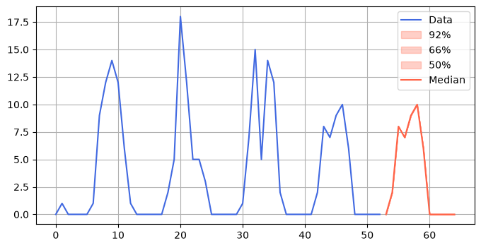
This is stark contrast to innovation-driven or conformal forecasts for a seasonal naive model.