Use a Custom Loss Function

Threedx lets you provide a custom loss function that it will minimize when fitting the model. The loss function takes two numpy vectors as input, the past observations y and one-step-ahead predictions y_hat of those training observations. It has to return a scalar loss value based on which Threedx then judges the predictions.

In the Get Started section you saw how a model is fitted using the mean absolute error loss function tdx.mae() provided by Threedx. Let’s recap this quickly here by importing Threedx and fitting it to the same example data.

import numpy as np
import threedx as tdx
from threedx.graphics import plot_forecast
from threedx._data import _load_y

y, y_future = _load_y()

model = tdx.Threedx(
    period_length=12,
    parameter_grid=tdx.initialize_parameters_at_random(
        size=2500,
        seed=729,
        include_edge_cases=True
    )
)

model = model.fit(
    y=y,
    loss=tdx.mae # <- The loss function is specified here!
)

sample_paths_of_mae_model = model.predict(
    horizon=12,
    n_samples=2501,
    observation_driven=True,
    draw=None,
    seed=388
)

The fitted model achieves a minimal loss (minimum absolute error) of:

model.minimal_loss

np.float64(1.4440626303029747)

Structure of a Loss Function

To specify your own loss, follow the provided example functions. For example, take a look at the function signature of tdx.mae():

tdx.mae

<function threedx.loss.mae(y_hat: numpy.ndarray[tuple[int], numpy.dtype[typing.Any]], y: numpy.ndarray[tuple[int], numpy.dtype[typing.Any]]) -> numpy.ndarray[tuple[typing.Literal[1]], numpy.dtype[numpy.floating]]>

The function fulfills the threedx.loss.Loss protocol.

What the protocol does not capture, however, are the following implicit promises and expectations:

• Both y_hat and y will be of identical dimensions

• Both y_hat and y will not be NaN

• The returned value of the loss must not be NaN

Define a New Loss Function

To demonstrate how you can define a new loss function, let’s implement the robust loss function described in section 3.1 and appendix A.5 of the Toto paper.

Assuming the preferred value of \(\delta = 0.1\), the authors define the loss as:

\[L_{\text{Robust(0,0.1)}}(y_t, \hat{y}_t) = \log ( \frac{1}{2}((y_t - \hat{y}_t) / 0.1)^2 + 1 )\]

This can be implemented as follows:

def robust_toto_loss(y_hat, y):
    losses = np.log(0.5 * (((y_hat - y) / 0.1) ** 2) + 1)
    return np.mean(losses)

The new robust_toto_loss() function accepts numpy vectors and returns a scalar:

robust_toto_loss(y_hat=y[0:12], y=y[12:24])

np.float64(3.584734759560734)

You can now refit the model using the new loss. When optimized using mean absolute error, the optimal parameters were:

print(f"{model.best_alpha=}")
print(f"{model.best_alpha_seasonal=}")
print(f"{model.best_alpha_seasonal_decay=}")

model.best_alpha=np.float64(0.0020794643341743354)
model.best_alpha_seasonal=np.float64(0.8592539151871426)
model.best_alpha_seasonal_decay=np.float64(0.1156035225969444)

Now refit the model and check whether using the new loss different parameters are optimal:

model_toto = model.fit(
    y=y,
    loss=robust_toto_loss
)

print(f"{model_toto.best_alpha=}")
print(f"{model_toto.best_alpha_seasonal=}")
print(f"{model_toto.best_alpha_seasonal_decay=}")

model_toto.best_alpha=np.float64(0.004292717950963551)
model_toto.best_alpha_seasonal=np.float64(0.9795816333414259)
model_toto.best_alpha_seasonal_decay=np.float64(0.2778912171864287)

These new parameters adjust the forecast closer to that of a Seasonal Naive model.

The forecast of the model optimized using the robust Toto loss looks as follows:

sample_paths_of_toto_model = model_toto.predict(
    horizon=12,
    n_samples=2501,
    observation_driven=True,
    draw=None,
    seed=388
)

plot_forecast(
    forecast=sample_paths_of_toto_model,
    y=y,
    y_future=y_future
)

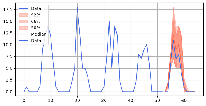
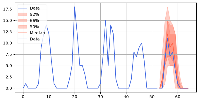
Overall, the prediction does not differ dramatically. The main difference when compared to the forecast from the MAE-optimized model (below) are the sharper forecast intervals which are a consequence of the model parameters that moved closer to those of a seasonal naive model.

plot_forecast(
    forecast=sample_paths_of_mae_model,
    y=y,
    y_future=y_future
)