Interpret a Threedx Model and its Forecasts

Everything about a Threedx model is interpretable, because

• its forecast is a linear combination of past observations,

• you chose the loss function the model was fitted to minimize,

• and the trialled parameter combinations are deterministic.

Let’s take a closer look at each of those aspects by fitting the model you’ve seen in the Get Started section and then inspecting it.

import numpy as np
import threedx as tdx
import matplotlib.pyplot as plt

np.set_printoptions(precision=3)
rng = np.random.default_rng(seed=512)

y = rng.poisson(
    lam=np.maximum(
        0.1,
        1 + 10 * np.sin(2 * np.pi * np.arange(6, 59) / 12)
    ),
    size=53
)

grid = tdx.initialize_parameters_at_random(
    size=2500,
    seed=729,
    include_edge_cases=True
)

model = tdx.Threedx(period_length=12, parameter_grid=grid)
model = model.fit(y=y, loss=tdx.mae)

sample_paths_from_observations = model.predict(
    horizon=12,
    # Using a very large number of samples to reduce the sampling error when
    # trying to reproduce the point prediction of the linear combination.
    # Not recommended in practice.
    n_samples=100_001,
    observation_driven=True,
    draw=None,
    seed=388
)

A Threedx Forecast as Linear Combination

One-Step-Ahead Prediction

The one-step-ahead forecast that Threedx.predict() generates is a linear combination of the past observations y and the weights assigned to them by the fitted model. The weights of a fitted model can be accessed via the .weights() method. They are aligned with the past observations y, so that the linear combination or dot-product of weights and y will equal the one-step-ahead point prediction.

print("one-step-ahead point prediction as linear combination of past observations:")
print(round(np.dot(model.weights(), y), 3))

print("")

print("one-step-ahead mean of sample paths as returned by .predict():")
print(round(np.mean(sample_paths_from_observations, axis=0)[0], 3))

# A small difference between the two values is unavoidable due to the sampling
# error introduced when drawing sample paths and then aggregating them.

one-step-ahead point prediction as linear combination of past observations:
0.295

one-step-ahead mean of sample paths as returned by .predict():
0.296

Given that the forecast is a linear combination of past observations and the model’s weights, it’s fair to make statements such as the following:

print(f"""
    The most recent observation contributes {round(model.weights()[-1]*100, 2)}%
    to the one-step-ahead prediction.
""")

print(f"""
    The observations of the most recent 12 months contribute
    {round(np.sum(model.weights()[(y.size-12):])*100, 2)}% to the one-step-ahead
    prediction.
""")

print(f"""
    If the observation a year ago had been 20 units larger,
    the one-step-ahead prediction would increase by
    {round(model.weights()[y.size-12]*20, 2)} units.
""")

    The most recent observation contributes 3.26%
    to the one-step-ahead prediction.


    The observations of the most recent 12 months contribute
    30.14% to the one-step-ahead
    prediction.


    If the observation a year ago had been 20 units larger,
    the one-step-ahead prediction would increase by
    4.53 units.

k-Step-Ahead Prediction

The same reasoning can be extended to all k-step-ahead predictions with the caveat that Threedx forecasts are recursive in that the two-step-ahead prediction is the linear combination of the past observations and the one-step-ahead prediction, and so on.

Accordingly, the weights expand during prediction to align with both past observations and previously created predictions. Those weights are not returned by .weights() but can be derived from the model’s parameters.

weights_for_one_step_ahead_prediction = model.weights()

weights_for_two_step_ahead_prediction = tdx.weights_threedx(
    alpha=model.best_alpha,
    alpha_seasonal=model.best_alpha_seasonal,
    alpha_seasonal_decay=model.best_alpha_seasonal_decay,
    # The `n` argument is the only difference between the one-step-ahead and the
    # two-step-ahead prediction. As the weights need to align with more
    # observations (as they now include predictions, too), `n` increases.
    n=y.size+1,
    period_length=12,
)

Depending on the fitted model and the number of past observations, weights don’t change by a lot as you expand them. In the case here, as little weight is assigned to the first observation, the weights barely change as they are expanded but rather shifted by one position. The most recent weight of 0.3259 will not be assigned to the most recent observation but to the first prediction.

print(np.concatenate(
    [np.zeros(shape=(1,)), weights_for_one_step_ahead_prediction]
))

print(weights_for_two_step_ahead_prediction)

[0.000e+00 7.021e-06 4.999e-05 3.559e-04 2.534e-03 1.804e-02 1.452e-01
 2.049e-02 2.889e-03 4.075e-04 5.747e-05 8.106e-06 1.143e-06 8.140e-06
 5.795e-05 4.126e-04 2.938e-03 2.092e-02 1.684e-01 2.375e-02 3.349e-03
 4.724e-04 6.663e-05 9.397e-06 1.325e-06 9.436e-06 6.719e-05 4.783e-04
 3.406e-03 2.425e-02 1.952e-01 2.753e-02 3.883e-03 5.477e-04 7.724e-05
 1.089e-05 1.537e-06 1.094e-05 7.789e-05 5.546e-04 3.948e-03 2.811e-02
 2.263e-01 3.192e-02 4.502e-03 6.349e-04 8.955e-05 1.263e-05 1.781e-06
 1.268e-05 9.030e-05 6.429e-04 4.577e-03 3.259e-02]
[9.861e-07 7.021e-06 4.999e-05 3.559e-04 2.534e-03 1.804e-02 1.452e-01
 2.049e-02 2.889e-03 4.075e-04 5.747e-05 8.106e-06 1.143e-06 8.140e-06
 5.795e-05 4.126e-04 2.938e-03 2.092e-02 1.684e-01 2.375e-02 3.349e-03
 4.724e-04 6.663e-05 9.397e-06 1.325e-06 9.436e-06 6.719e-05 4.783e-04
 3.406e-03 2.425e-02 1.952e-01 2.753e-02 3.883e-03 5.477e-04 7.724e-05
 1.089e-05 1.537e-06 1.094e-05 7.789e-05 5.546e-04 3.948e-03 2.811e-02
 2.263e-01 3.192e-02 4.502e-03 6.349e-04 8.955e-05 1.263e-05 1.781e-06
 1.268e-05 9.030e-05 6.429e-04 4.577e-03 3.259e-02]

You can now recompute the linear combination using the expanded set of weights to derive the two-step-ahead prediction. First calculate the one-step-ahead prediction and concatenate it with past observations. Then use the extended history in a second dot product to arrive at the two-step-ahead prediction.

Comparing the two-step-ahead prediction against the mean of the two-step-ahead sample paths, results match closely.

one_step_ahead_prediction = np.zeros((1,))
one_step_ahead_prediction[0] = np.dot(model.weights(), y)

print("two-step-ahead point prediction as linear combination of past observations:")
print(round(
    np.dot(
        weights_for_two_step_ahead_prediction,
        np.concatenate([y, one_step_ahead_prediction])
    ),
3))

print("")

print("two-step-ahead mean of sample paths as returned by .predict():")
print(round(np.mean(sample_paths_from_observations, axis=0)[1], 3))

# A small difference between the two values is unavoidable due to the sampling
# error introduced when drawing sample paths and then aggregating them.

two-step-ahead point prediction as linear combination of past observations:
2.098

two-step-ahead mean of sample paths as returned by .predict():
2.091

Visualize the Weights

It can be difficult to interpret the weights when the values are printed as above. Consider visualizing the weights using a barplot or similar methods. That makes it easy to see which past observations are weighted heavily by the model.

The plot below highlights that the seasonal average component dominates the model fitted above. Every prediction is primarily an average of past observations at the same point in the seasonal period. Weights are tilted slightly in favor of more recent observations.

plt.bar(
    x=np.arange(0, weights_for_one_step_ahead_prediction.size, step=1),
    height=weights_for_one_step_ahead_prediction,
)

<BarContainer object of 53 artists>

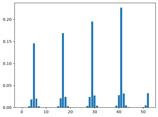
You should expect these weigths due to the large alpha_seasonal parameter of the fitted model (leading to the seasonal peaks) combined with a very small but not zero alpha parameter and a small alpha_seasonal_decay parameter, both contributing to decreasing weights for older observations.

print(f"{model.best_alpha=}")
print(f"{model.best_alpha_seasonal=}")
print(f"{model.best_alpha_seasonal_decay=}")

model.best_alpha=np.float64(0.0020794643341743354)
model.best_alpha_seasonal=np.float64(0.8592539151871426)
model.best_alpha_seasonal_decay=np.float64(0.1156035225969444)

Parameter Combinations and Loss Function

It is unusual that Threedx does not use the loss function’s gradients to fit the model’s parameters. But with only three parameters, all constrained to a 0-to-1 range, to fit, it is not unreasonable to simply evaluate a grid of parameter combinations and pick the one that worked best (i.e., minimized the loss function). Yes, there is a good chance that there exists another parameter combination that would achieve a slightly improved training loss. But both parameter values and the resulting predictions are unlikely to differ much as long as a fairly exhaustive set of parameter combinations was trialled.

A similar idea was used in “A white-boxed ISSM approach to estimate uncertainty distributions of Walmart sales” (2021).

This provides an advantage in that it allows us to state with certainty that, within the set of trialled parameter combinations, we did indeed find the set of parameters that minimizes the loss function. In contrast, with other approaches of optimization, there is a chance of ending up in a weird local minimum without realizing it.

You can inspect the minimal training loss achieved by the fitted parameters:

print(f"{model.minimal_loss=}")

model.minimal_loss=np.float64(1.4440626303029747)

Or you could print all losses of all trialled parameter combinations:

print(model.losses)

[2.732 4.217 1.518 ... 3.311 3.101 2.639]

This loss vector is aligned with the trialled parameter combinations, so you could, for example, print the first six parameter combinations and their corresponding losses:

print(grid[0:6,])
print(model.losses[0:6])

[[1.    0.    0.   ]
 [0.    0.    0.   ]
 [0.    1.    0.   ]
 [0.    1.    1.   ]
 [0.    0.    1.   ]
 [0.629 0.262 0.435]]
[2.732 4.217 1.518 1.976 4.236 3.021]

Which shows that from the five edge cases, the third (seasonal average) performs best, while the fifth (average of last 12 observations) performs worst. The fourth (seasonal naive) comes closest to the third.

Additionally, the minimal training loss printed above (1.444) is not that much better than what the seasonal average achieves (1.518). In fact, given how the example series was created, the seasonal average is the correct model, but the observation noise leads to slightly different parameters—though still dominated by the seasonal average component, as you saw above.