Generating Diverse Weights for Training

set.seed(4729)
library(threedx)
library(ggplot2)

Parameter Space and Weights Space

During training of a threedx model, the parameters alpha, alpha_seasonal, and alpha_seasonal_decay are translated into weights that are assigned to every index of the observed time series.

For example, given a time series of n = 50 observations with period length period_length = 12L, and parameter choices alpha = 0.9, alpha_seasonal = 0.9, and alpha_seasonal_decay = 0.05, the resulting weights would be:

weights_first <- weights_threedx(
  alpha = 0.9,
  alpha_seasonal = 0.9,
  alpha_seasonal_decay = 0.05,
  n = 50L,
  period_length = 12L
)

round(tail(weights_first, 13L), 4)
#>  [1] 0.0000 0.0000 0.0000 0.0000 0.0000 0.0000 0.0000 0.0000 0.0000 0.0000
#> [11] 0.0001 0.0099 0.9900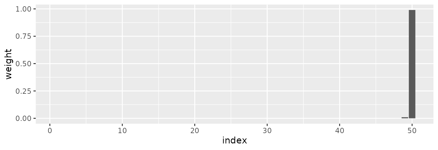

We would expect that, if we let the model train over a wide range of possible parameter combinations, we will try many different combinations of weights and cover the range of possible models, and thereby find a good one.

But the following set of parameters–at the other end of the possible alpha_seasonal spectrum–results in nearly identical weights:

weights_second <- weights_threedx(
  alpha = 0.9,
  alpha_seasonal = 0.1,
  alpha_seasonal_decay = 0.05,
  n = 50L,
  period_length = 12L
)

round(tail(weights_second, 13L), 4)
#>  [1] 0.0000 0.0000 0.0000 0.0000 0.0000 0.0000 0.0000 0.0000 0.0001 0.0007
#> [11] 0.0074 0.0819 0.9100

And so does this third combination of parameters where alpha_seasonal_decay is at the opposite end of its allowed range:

weights_third <- weights_threedx(
  alpha = 0.9,
  alpha_seasonal = 0.1,
  alpha_seasonal_decay = 0.95,
  n = 50L,
  period_length = 12L
)

round(tail(weights_third, 13L), 4)
#>  [1] 0.0000 0.0000 0.0000 0.0000 0.0000 0.0000 0.0000 0.0000 0.0001 0.0007
#> [11] 0.0074 0.0819 0.9100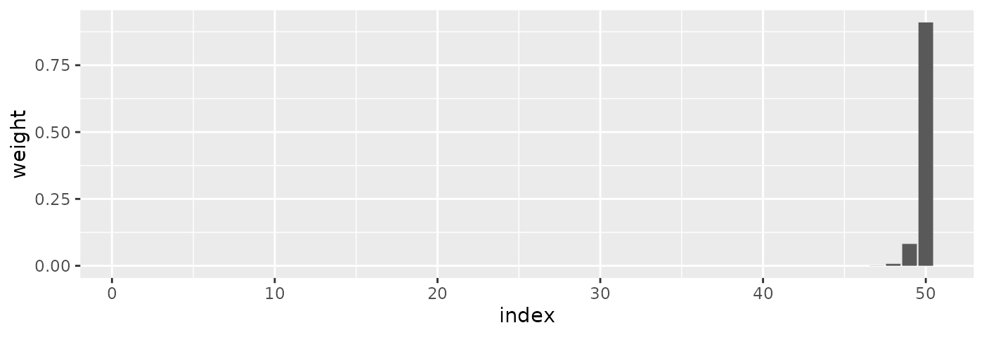

Thus, large changes in the parameter space do not necessarily imply large changes in the weights space. Since the weights space is what we ultimately care about, and since we would like to cover the weights space perhaps uniformly by default, this means that covering the parameter space in a uniform manner is suboptimal.

The Impact of alpha

As indicated by the examples above, the alpha parameter can overshadow the other two parameter choices. Depending on the length of the period and the time series, alpha will assign so much weight to the most recent one, two, or three indices that there simply is no weight left for any other indices that come later—those that are heavily impacted by the choice of alpha_seasonal and alpha_seasonal_decay.

This can render the grid generated by the default list_sampled_alphas() function wasteful, as it uniformly samples the parameter space, thereby trying many different combinations of alpha_seasonal and alpha_seasonal_decay for alpha values that will lead to essentially equal set of weights.

Let’s take a look what would happen with a usual call to list_sampled_alphas() that samples the entire [0, 1]-cube uniformly.

Below code chunk starts by creating the alphas_grid. Once the alphas_grid is created, we generate the set of 1000 weights implied by the 1000 different parameter combinations. For each of the 1000 implied sets of weights, we take the three weights assigned to the three most recent observations and sum them, resulting in the vector weight_three_most_recent_indices of length 1000. Each value summarizes the probability that a parameter set assigns to the three most recent indices.

alphas_grid <- list_sampled_alphas(
  n_target = 1000L,
  alpha_lower = 0.0001,
  alpha_upper = 0.9999,
  alpha_seasonal_lower = 0.0001,
  alpha_seasonal_upper = 0.9999,
  alpha_seasonal_decay_lower = 0.0001,
  alpha_seasonal_decay_upper = 0.9999,
  oversample_lower = 0,
  oversample_upper = 0
  )

weight_three_most_recent_indices <- rowSums(
  threedx:::weights_threedx_vec(
    alphas = alphas_grid$alpha,
    alphas_seasonal = alphas_grid$alpha_seasonal,
    alphas_seasonal_decay = alphas_grid$alpha_seasonal_decay,
    n = 50L,
    period_length = 12L
  )[, 48:50]
)

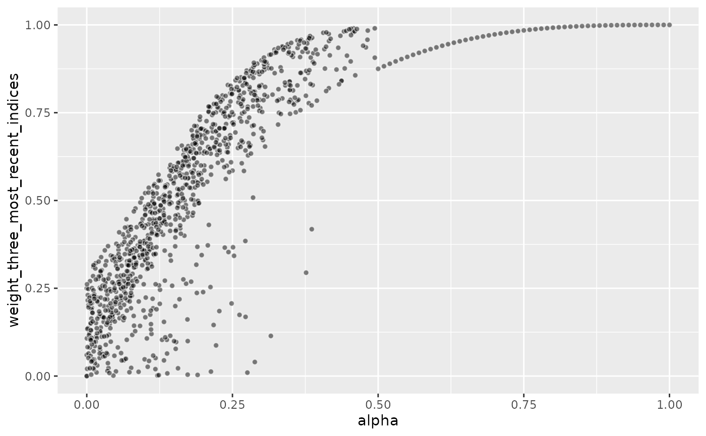
The graph below shows how the choice of alpha drives the (share of the total) weight assigned to the three most recent observations alone.

Since the three parameters are sampled uniformly and independently from each other, roughly 25% of parameter combinations plotted below will have an alpha larger than 0.75, 50% will have an alpha larger than 0.5, and so on.

Consequently, half of the parameter combinations assign more than 80% of weight to the three most recent observations, and roughly 25% of the parameter combinations even assign nearly 100% weight to the three most recent indices.

Each of the 1000 parameter combinations implies a different model, and thus different predictions, each of which leads to different forecast performance. But since half of the parameter combinations imply very similar weights, with the three most recent observations being the only ones impacting the forecast, half of the models that are evaluated produce very similar forecasts.

Generating More Diverse Weights

With learn_weights(), the model is trained via grid search. The provided alphas_grid is evaluated, and the loss minimizing parameter combination is chosen. For fast performance, we want to keep alphas_grid as small as possible. For improved forecast performance, we want to try an as wide alphas_grid as possible. But we especially don’t want to try parameter combinations that imply similar weights multiple times and are close to duplicate.

Given the above, we don’t need to try different values of alpha_seasonal and alpha_seasonal_decay for different alpha values. As soon as alpha is moderately large, the weights will be essentially those of simple exponential smoothing anyway.

Something like the following could help.

First, we create a simple sequence of moderately large alpha values (here, larger than 0.50) while holding the other two constant:

alphas_grid_ses <- data.frame(
  alpha = seq(0.50, 1, by = 0.01),
  alpha_seasonal = 0,
  alpha_seasonal_decay = 0
)

Next, we draw a large set of random values of all three parameters but keep alpha below 0.25:

alphas_grid <- data.frame(
  alpha = rbeta(n = 1000, 1, 2) * 0.50,
  alpha_seasonal = rbeta(n = 1000, 0.75, 0.75),
  alpha_seasonal_decay = rbeta(n = 1000, 0.7, 0.8)
)

Finally we take the edge case parameter combinations and union the three different sets:

alphas_grid <- unique(
  rbind(
    list_edge_alphas(),
    alphas_grid_ses,
    alphas_grid
    )
  )

weight_three_most_recent_indices <- rowSums(
  threedx:::weights_threedx_vec(
    alphas = alphas_grid$alpha,
    alphas_seasonal = alphas_grid$alpha_seasonal,
    alphas_seasonal_decay = alphas_grid$alpha_seasonal_decay,
    n = 50L,
    period_length = 12L
  )[, 48:50]
)

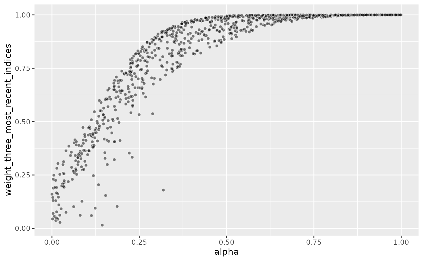
As is visible in the resulting graph, there are now a lot more samples at the smaller weight levels for the three most recent observations. This should help to leave more samples for parameter combinations that model interesting combinations of seasonal patterns.