Fit a 3DX model to a time series

Returns a threedx model applied to time series y after learning the optimal set of parameters by minimizing a provided loss function. Use predict.threedx() to generate a forecast based on the fitted model.

Usage

learn_weights(
  y,
  period_length,
  alphas_grid,
  loss_function,
  penalize = FALSE,
  loss_increase = 1
)

Arguments

y

The time series to be forecasted as numeric vector (not as ts() object)

period_length

The presumed length of y's seasonal period; for example, 12L for monthly observations, 7L for daily observations, ...

alphas_grid

A data frame of possible parameter combinations to generate the weights of the final model. The optimal parameter set will be chosen based on the minimization of loss_function. The expected columns are numeric and called alpha, alpha_seasonal, alpha_seasonal_decay. At least one row must be provided. All values must be between 0 and 1. Use, for example, list_sampled_alphas() or list_edge_alphas() to generate this data frame, or generate it in any way you like.

loss_function

A function with first argument y_hat and optionally more arguments. Usually, to compute a loss, at least an additional y argument is required to compute errors. Must be able to handle additional parameters via ... to allow for potential future changes in the set of arguments passed to loss_function by learn_weights(). For examples, see loss_mae() or loss_mae_with_observation_weight(). It can be assumed that the arguments y_hat and y passed by learn_weights() are numeric vectors of equal length. The provided loss_function must return a numeric scalar value.

penalize

Logical, FALSE by default. If TRUE, will try to pick a set of parameters that are simpler while not increasing the loss too much. The allowed increase in loss in percentage points is defined via the loss_increase. A model is simpler if more of its parameters are equal to exactly zero or one, as these correspond to the edge cases.

loss_increase

A non-negative scalar value by which the loss may be increased compared to the best possible loss, in percentage points. This argument is ignored unless penalize = TRUE. The default of 1 corresponds to a range of up to a 1 percentage point increase in loss.

Value

A fitted model object of class threedx, which is a list of:

• A numeric vector weights of the same length as the input y, assigning a weight to each index of the past observations. The weights sum to 1. These weights are the fitted weights used to produce forecasts.

• A numeric scalar alpha, the optimal paramater for the exponential smoothing component chosen during model training

• A numeric scalar alpha_seasonal, the optimal paramater for the seasonal exponential smoothing component chosen during model training

• A numeric scalar alpha_seasonal_decay, the optimal paramater for the seasonal exponential decay smoothing component chosen during model training

• A numeric vector fitted containing fitted values for each index of y; the up to period_length-first observations may be missing.

• A numeric vector residuals containing the residuals for the training data as computed by y - fitted, thus the up to period_length-first observations may be missing.

• A numeric vector y, the input y

• A scalar n, the number of observations provided via y

• A scalar period_length, the input period_length

• A function loss_function, the provided loss_function

• A scalar loss, the value computed by the provided loss_function based on the input y and the fitted values (ignoring the initial missing values) for the loss minimizing set of parameters reported in alpha, alpha_seasonal, alpha_seasonal_decay

• A logical penalize, identical to the provided function argument

• A scalar loss_increase, identical to the provided function argument

• A list full containing intermediate results observed during model optimization for all other parameter combinations provided via alphas_grid

See also

predict.threedx(), list_sampled_alphas(), loss_mae()

Examples

set.seed(9284)
y <- stats::rpois(n = 55, lambda = pmax(0.1, 1 + 10 * sinpi((5 + 1:55 )/ 6)))

alphas_grid <- list_sampled_alphas(
  n_target = 1000L,
  include_edge_cases = TRUE
)

model <- learn_weights(
  y = y,
  alphas_grid = alphas_grid,
  period_length = 12L,
  loss_function = loss_mae
)

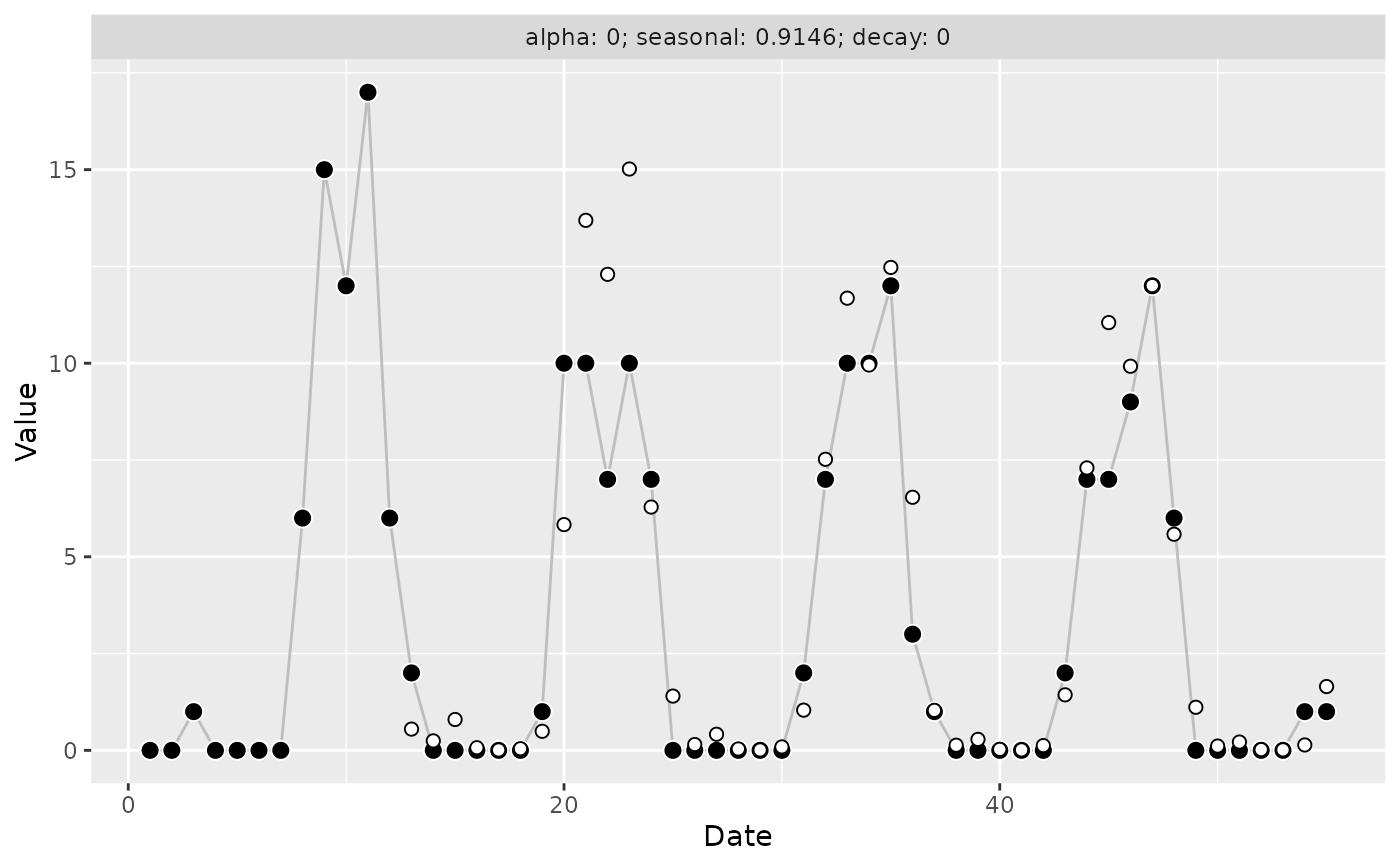
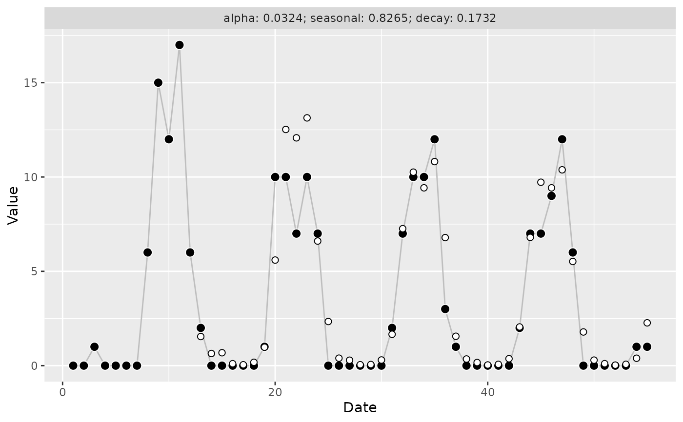
if (require("ggplot2")) {
  autoplot(model)
}
#> Loading required package: ggplot2


model_penalized <- learn_weights(
  y = y,
  alphas_grid = alphas_grid,
  period_length = 12L,
  loss_function = loss_mae,
  penalize = TRUE,
  loss_increase = 10
)

model$full$best_alphas
#>        alpha alpha_seasonal alpha_seasonal_decay
#> 1 0.03240655      0.8265107             0.173151
model_penalized$full$best_alphas
#>   alpha alpha_seasonal alpha_seasonal_decay
#> 1     0      0.9146342                    0

if (require("ggplot2")) {
  autoplot(model_penalized)
}