Draw forecast sample paths from a fitted 3DX model

Usage

# S3 method for threedx
predict(
  object,
  horizon,
  n_samples,
  observation_driven,
  innovation_function,
  postprocess = identity,
  ...
)

Arguments

object: A fitted model object of class threedx
horizon: An integer defining the forecast horizon
n_samples: An integer defining the number of sample paths to draw
observation_driven: Logical; if TRUE, sample paths are generated by drawing from weighted historical observations directly instead of adding innovation noise on the current mean forecast. This is similar to the Non-Parametric Time Series forecaster (NPTS) described in "GluonTS: Probabilistic Time Series Models in Python" (2019) by Alexandrov et al. (see https://arxiv.org/abs/1906.05264). If FALSE, sample paths will be generated by adding innovation noise on top of the current weighted average forecast.
innovation_function: A function with arguments n and errors. Must be able to handle additional parameters via ... to allow for potential future changes in the set of arguments passed to innovation_function by predict.threedx(). For examples, see draw_normal_with_drift() or draw_bootstrap_weighted(). The provided innovation_function must return a numeric vector of length n that contains i.i.d samples that can be used for any sample path and forecast horizon. This argument is ignored when observation_driven=TRUE.
postprocess: A function that is applied on a numeric vector of drawn samples for a single step-ahead before the samples are used to update the state of the model, and before outliers are removed (if applicable). By default equal to identity(), but could also be something like function(x) pmax(x, 0) to enforce a lower bound of 0, or any other transformation of interest that returns a numeric vector of equal length as that of the input. Note that this can cause arbitrary errors caused by the author of the function provided to postprocess. For examples, see to_non_negative_with_identical_mean() or to_moment_matched_nbinom().
...: Additional arguments passed to innovation_function

Value

A forecast object of class threedx_paths, which is a list of:

A paths numeric matrix of dimensions n_samples-times-horizon. The matrix stores the forecast sample paths that are the probabilistic forecast returned by the threedx model. Aggregate across the first dimension to derive expectations of the forecast distribution, aggregate across the second dimension to derive sums over the forecast horizon.
The input horizon argument
The input n_samples argument
The input observation_driven argument
The model model provided via object, an object of class threedx

Details

While observation_driven can be effective at forecasting wide ranges of time series, the induced forecast distribution collapses to a single point as alpha, alpha_seasonal, and alpha_seasonal_decay values tend towards 1. While the corresponding point prediction may still be optimal, the uncertainty in the forecast is likely underestimated.

For example, if alpha = 0.98, alpha_seasonal=0, and alpha_seasonal_decay=0, the resulting forecast distribution assigns 98% probability to the most recent observation, thus collapsing most prediction intervals onto that point. This can be highly unrealistic for time series whose level is changing rapidly and therefore require large alpha values.

To circumvent this issue, one can design certain conditions under which observation_driven is set to TRUE. For example, using k_largest_weights_sum_to_less_than_p_percent(), one can check that the learned model assigns weight to at least a few observations, and only then set observation_driven=TRUE. However, if the underlying time series is truly a random walk, observation_driven=TRUE will always be a poor choice as it limits the range of possible future values too much.

Examples

set.seed(9284)
y <- stats::rpois(n = 55, lambda = pmax(0.1, 1 + 10 * sinpi((5 + 1:55 )/ 6)))

model <- learn_weights(
  y = y,
  alphas_grid = list_sampled_alphas(
    n_target = 1000L,
    include_edge_cases = TRUE
  ),
  period_length = 12L,
  loss_function = loss_mae
)

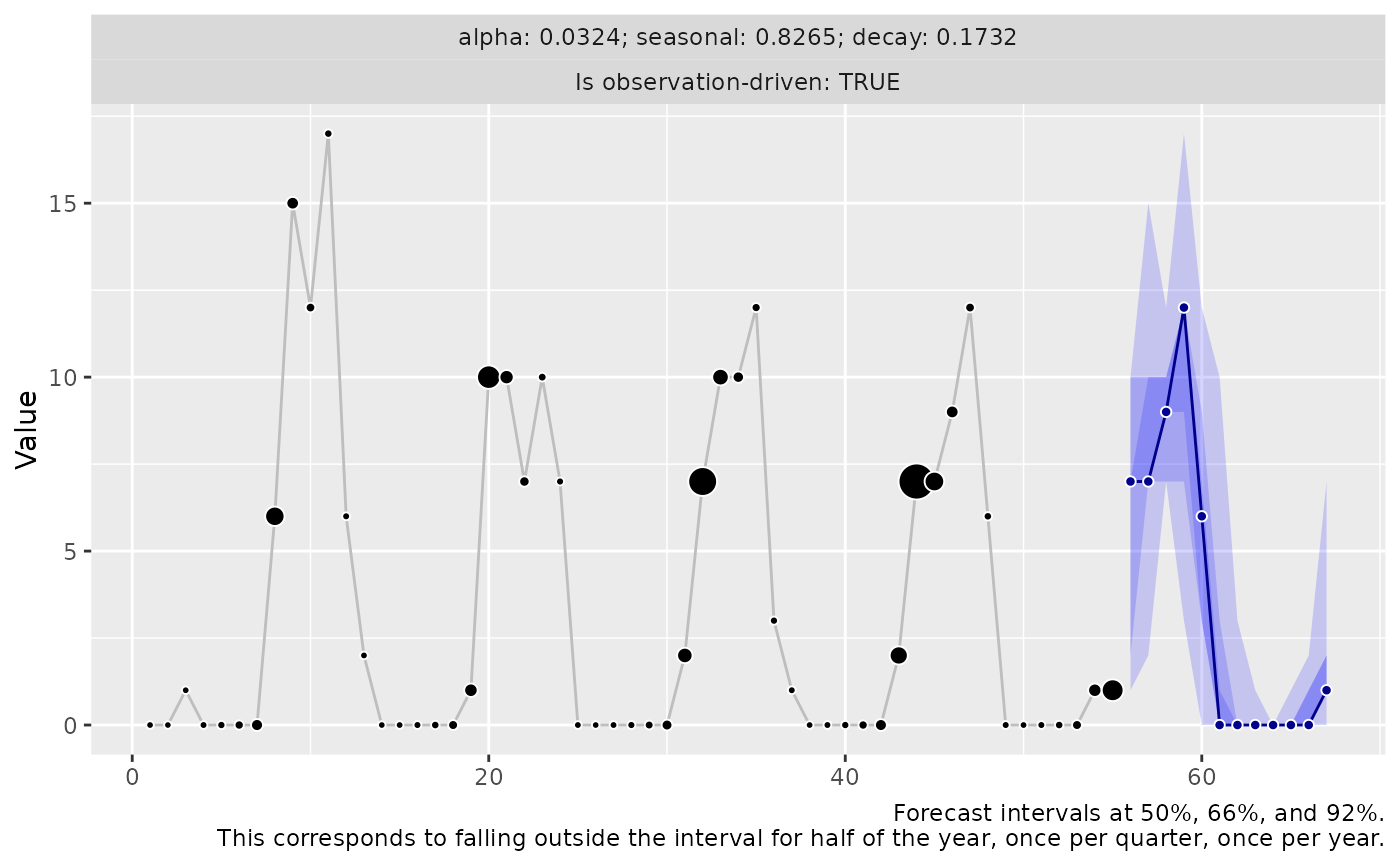
forecast_observation_driven <- predict(
  object = model,
  horizon = 12L,
  n_samples = 2500L,
  observation_driven = TRUE
)

if (require("ggplot2")) {
  autoplot(forecast_observation_driven)
}


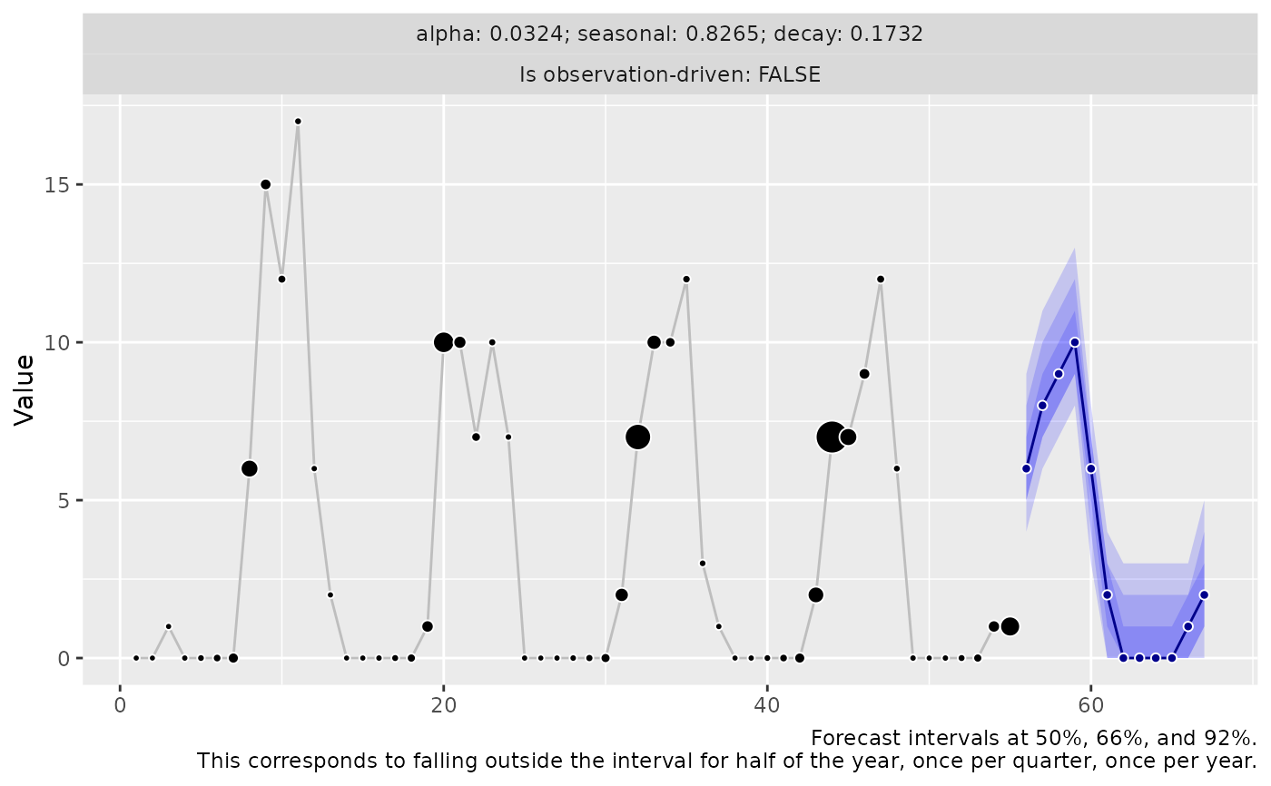
forecast_latent <- predict(
  object = model,
  horizon = 12L,
  n_samples = 2500L,
  observation_driven = FALSE,
  innovation_function = draw_bootstrap
)

if (require("ggplot2")) {
  autoplot(forecast_latent)
}


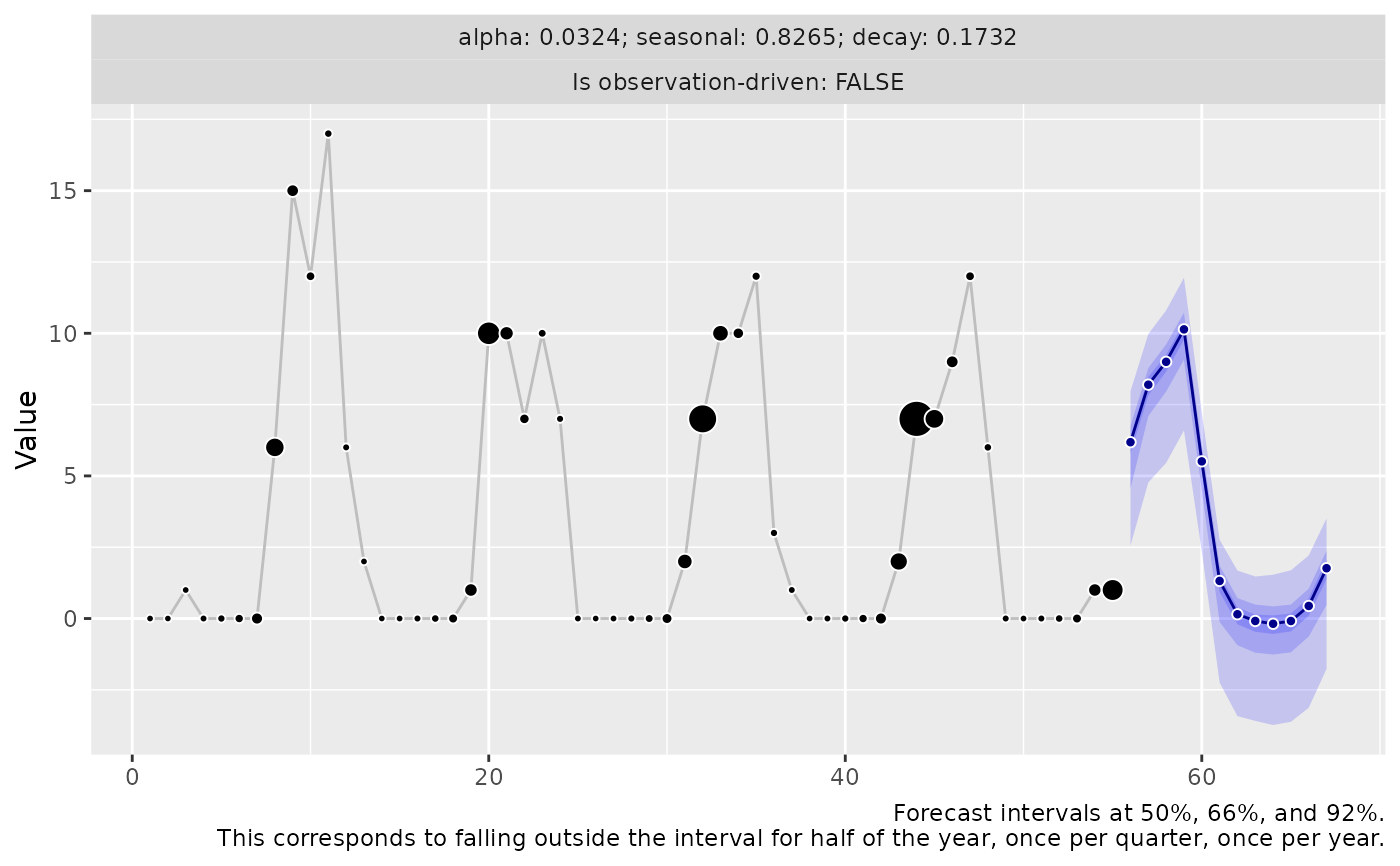forecast_latent_with_postprocessing <- predict(
  object = model,
  horizon = 12L,
  n_samples = 2500L,
  observation_driven = FALSE,
  innovation_function = draw_normal_with_zero_mean,
  postprocess = function(x) round(pmax(x, 0))
)

if (require("ggplot2")) {
  autoplot(forecast_latent_with_postprocessing)
}